Predicting respiratory motion using online learning of recurrent neural networks for safer lung radiotherapy

Photo by National Cancer Institute on Unsplash

There were approximately 2 million new lung cancer cases worldwide in 2020, and the 5-year relative survival rate of lung cancer patients is slightly above 22% [1,2]. This motivates research in lung radiotherapy, and AI is one of the tools that is being utilized toward that goal. Have you ever wondered how AI could improve lung cancer treatment? And why recurrent neural networks (RNN) in particular may be helpful for that task? Also, what is online learning, and why is this particularly useful in that context? Here, I will do my best to answer these questions by summarizing my recent research article "Prediction of the position of external markers using a recurrent neural network trained with unbiased online recurrent optimization for safe lung cancer radiotherapy" published in "Computer methods and programs in biomedicine" and presenting its main findings [3].

Please feel free to read the original article if you are curious and leave a comment. The accepted manuscript version is freely accessible on Arxiv. In case you are new to machine learning, please note that I may not explain all the basic concepts of that field here. As a result, the technical part might be challenging to go through. Still, I will try to explain the essential ideas clearly while skipping details. If you have already read my published article, this can still be of interest to you, as I cover the topic differently here by discussing additional minor results, the practical implementation in Matlab, as well as the rank-one trick that is at the heart of unbiased online recurrent optimization (UORO).

1. Why we need time series forecasting in lung radiotherapy

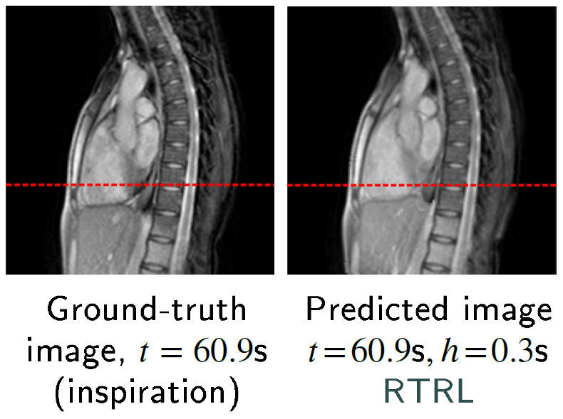
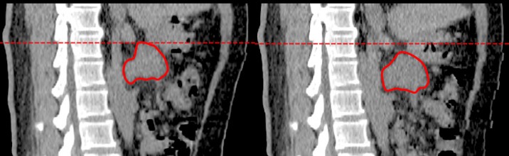
Lung tumors move with the respiratory motion. Hence, it is challenging to target them precisely, as real-time imaging during the radiotherapy treatment has limitations.

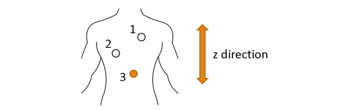
External markers are metallic objects placed on the chest that can help infer the position of tumors in the chest using spatial regression models, also called correspondence models.

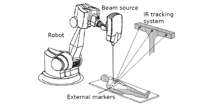
Even with infrared tracking of external markers, the position of tumors is difficult to estimate accurately because of the inaccuracies inherent to these internal-external correspondence models but also because treatment systems are subject to latencies due to image acquisition, robotic control, and radiation beam activation. That delay can prevent effective tumor irradiation and lead to excessive dose delivery to healthy tissues, leading to side effects such as pneumonitis, a condition that can become life-threatening.

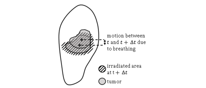
To address the issue of system delays, one can forecast the tumor position using past respiratory data. In the case of external guidance with markers as described above, we can predict the markers' positions.

2. Our approach

2.1. The dataset

In this study, I used the ExtMarker dataset comprising nine sequences with the 3D position of three external markers on the chest of healthy individuals. The sampling frequency is 10 Hz, and the movement amplitude in the spine direction is between 6mm and 40mm. That dataset is public and more information can be found in [7]. We divide the data for each sequence into training, cross-validation, and test sets.

Forecasting respiratory motion is challenging, as the breathing characteristics such as amplitude and period vary within each record, even though it appears predominantly cyclic. In addition, the individuals were asked to talk or laugh in approximately half of the records, which makes the task more complex. In real-world situations, sudden respiratory abnormalities such as coughing, hiccuping or yawning can also happen, which is why including challenging records is beneficial.

2.2 Let's dive into the world of RNNs.

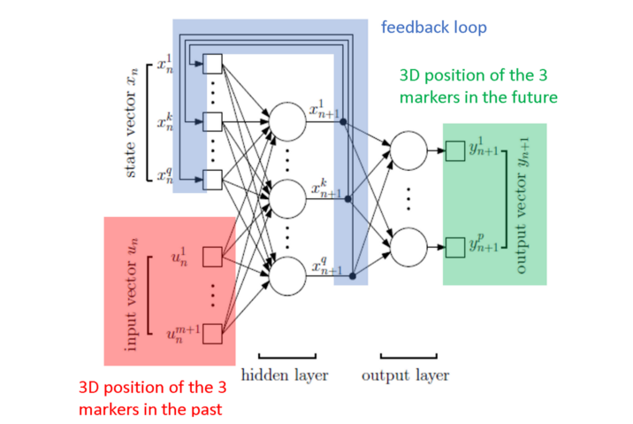
RNNs are a specific type of neural network equipped with a feedback loop enabling them to remember information acquired over time. As we perform forecasting, the position of the markers in the past and the future are respectively the input and the output of the network. Forecasting is a self-supervised learning problem, as manual annotation is not needed. This study uses a simple vanilla architecture with a single hidden layer.

RNNs are typically trained offline using back-propagation through time (BPTT). Offline learning designates a learning process in which there are two separate steps for training and inference. In our study, we use online learning instead, which means that training and inference are performed simultaneously. In the context of radiotherapy, this enables the network to adapt to unseen respiratory patterns despite having seen only limited data. Indeed, data collection for medical applications of AI is often difficult due to regulations about personal information protection. This study investigates the efficiency of UORO [8], a recent approach to online learning with RNNs, to forecast respiratory motion.

Let's briefly discuss how UORO works. First, let's write the RNN equations. The first equation below (state equation) describes the evolution of the internal state vector xₙ, and the second equation (measurement equation) enables calculating the output vector yₙ₊₁. θₙ and uₙ respectively designate the parameter vector and the input vector. Note that the parameter vector depends on n because we perform online learning.

\[ x_{n+1} = F_{st}(x_n, u_n, \theta_n) \]

\[ y_{n+1} = F_{out}(x_n, u_n, \theta_n) \]

The loss function that we seek to minimize is:

\[ L_{n} = \frac{1}{2} \|e_n\|_2^2 \]

In this equation, yₙ* designates the ground-truth labels (the positions of the markers that we want to predict). We can calculate the derivative of the loss with respect to θ using the definition of yₙ and the chain rule:

\[ \frac{\partial{L_{n+1}}}{\partial \theta} = \frac{\partial{L_{n+1}}}{\partial y}(y_{n+1}) \left[ \frac{\partial{F_{out}}}{\partial x}(x_n, u_n, \theta_n) \frac{\partial{x_n}}{\partial \theta} + \frac{\partial{F_{out}}}{\partial \theta}(x_n, u_n, \theta_n) \right] \]

Similarly, we can derive the following equation by using the chain rule with the measurement equation:

\[ \frac{\partial{x_{n+1}}}{\partial \theta} = \frac{\partial{F_{st}}}{\partial x}(x_n, u_n, \theta_n) \frac{\partial{x_n}}{\partial \theta} + \frac{\partial{F_{st}}}{\partial \theta}(x_n, u_n, \theta_n) \]

The first equation enables calculating the loss gradient as a function of the influence matrix ∂xₙ/∂θ. The second equation lets us update the influence matrix recursively at each time step. All the other partial derivatives can be computed using the definitions of the loss L and the chosen functions Fₒᵤₜ and Fₛₜ for our particular network; in our work, the latter are respectively a linear function and the element-wise hyperbolic tangent. That way of computing the loss gradient at each time step is called real-time recurrent learning (RTRL). The main drawback of RTRL is its high computational expense, as the update cost is O(q⁴), where q is the number of hidden units. This is due in particular to the size of the influence matrix, which has many entries that we need to update at each time step. The main idea of UORO is to estimate that matrix as the product of two random vectors (in other words, it is approximated by an unbiased rank-1 matrix estimator) and to update them at each time step:

\[ \mathbb{E}(\tilde{x}_n \tilde{\theta}_n^T) = \partial{x_n}/ \partial \theta_n \]

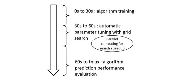
Again, I will not describe how these two vectors are updated here in detail. The important point is that there is an efficient way to compress the information contained in the influence matrix that enables reducing the computational cost down to O(q²). I will describe the mathematical property at the core of UORO in a bonus section at the end of the article, so please make sure to follow along :) In this research, I performed prediction independently for each sequence and conducted cross-validation using grid search.

2.3. UORO implementation in Matlab

Let's try to understand the basic implementation of UORO in Matlab. Here, I will describe the rnn_UORO function of the Github repository corresponding to my paper. If you have some knowledge of Python, there is nothing to be afraid of here, as the syntax of these two languages is very close to one another. You can skip this part if you are not interested in the code or prefer jumping to the analysis of the results.

As a side note, I would also like to mention the in-depth guide on realpython.com, entitled "MATLAB vs Python: Why and How to Make the Switch", which compares Matlab and Python and helped me a lot learning Python from my experience in Matlab (which are very similar languages anyway). You can also read that if you are proficient in Python and want to understand the Matlab syntax better.

First, I defined an auxiliary function to implement forward propagation according to the state equation (cf section 2.2). Functions in Matlab are defined using the function keyword, whereas the def keyword is used in Python. In this code, myRNN is a Matlab structure array (this is more or less the equivalent of a dictionary in Python and a structure in C) containing the RNN parameters. I chose the activation function phi as the hyperbolic tangent function. It is implemented using an anonymous function, which is the equivalent of a lambda function in Python.

I also used another auxiliary function to perform one gradient descent step with clipping at each time step. Here, theta is the RNN parameter vector, and dtheta is the loss gradient. Experimentally, I found that clipping helps stabilize the behavior of the RNN and achieve better performance. If you look at my code in the Github repository, you will notice that I also implemented adaptive moment estimation (ADAM). However, I experimentally noticed that the latter did not improve the forecasting accuracy. Therefore I only reported the results obtained with gradient descent in my article.

The main function for training the RNN takes as input the structures myRNN and pred_par, containing respectively the RNN parameters and the prediction hyper-parameters, as well as the 2D arrays Xdata and Ydata containing the input and output data (the positions of the markers).

First, we define variables containing helpful information, such as the size of our arrays (lines 3 to 11).

Then we loop over the time steps and perform forward propagation using the auxiliary function RNNstate_fwd_prop above (lines 13 to 21). These lines include the computation of yₙ₊₁ using the measurement equation (with a linear output function) and the instantaneous error (cf section 2.2). The tic function is used to tell the computer to "start the stopwatch" to measure the computation time corresponding to the current time step.

The portion of code between line 23 and line 45 is where things get quite mathematical. I will not go into the details here, but I will explain what happens from an overall point of view. First, you can see that there is a vector nu initialized randomly using the rand function (line 30). The important point here is that two vectors myRNN.xtilde and myRNN.theta_tilde are calculated from that random vector (lines 44 and 45). These correspond to the two random vectors that we mentioned in section 2.2 and whose product is an unbiased estimate of the influence matrix ∂xₙ/∂θ. You can see that they are recursively updated at each time step. Another important line is the computation of the loss gradient estimate gtilde from these two vectors (line 27). If you are interested in the underlying math, I would like to refer you to the original paper about UORO [8] and my article [3], which is the first to provide closed-form expressions for myRNN.dtheta, myRNN.dtheta_g, and dx in the case of vanilla RNNs. These are used in this implementation to compute the loss gradient. Also, there is a bonus section at the end of this story covering the basic mathematical property that UORO relies on, so stick with me :)

Finally, we update the gradient estimate with the update_param_optim auxiliary function described above (line 51). I used the reshape function and slicing, as the weight matrices myRNN.Wa, myRNN.Wb, and myRNN.Wc are hard-coded as 2D arrays and the vector theta_vec concatenating these weights is a line vector. In the end, I update the state vector and store the calculation time (with toc) and the instantaneous loss for later analysis.

The code in my Github repository differs slightly as it also handles GPU computing, but I skipped that part to make explanations simple. Also, I experimentally found that using my GPU made the UORO calculations slower. Therefore, my article only reports the performance of UORO corresponding to CPU calculations.

3. Results

3.1. Qualitative observation of the forecasting behavior

Let's first define essential terms here. We call "horizon" and denote by h the time interval in advance for which the prediction is made, and signal history length (SHL) the interval of time, the information of which is used to make a single prediction at a given time step.

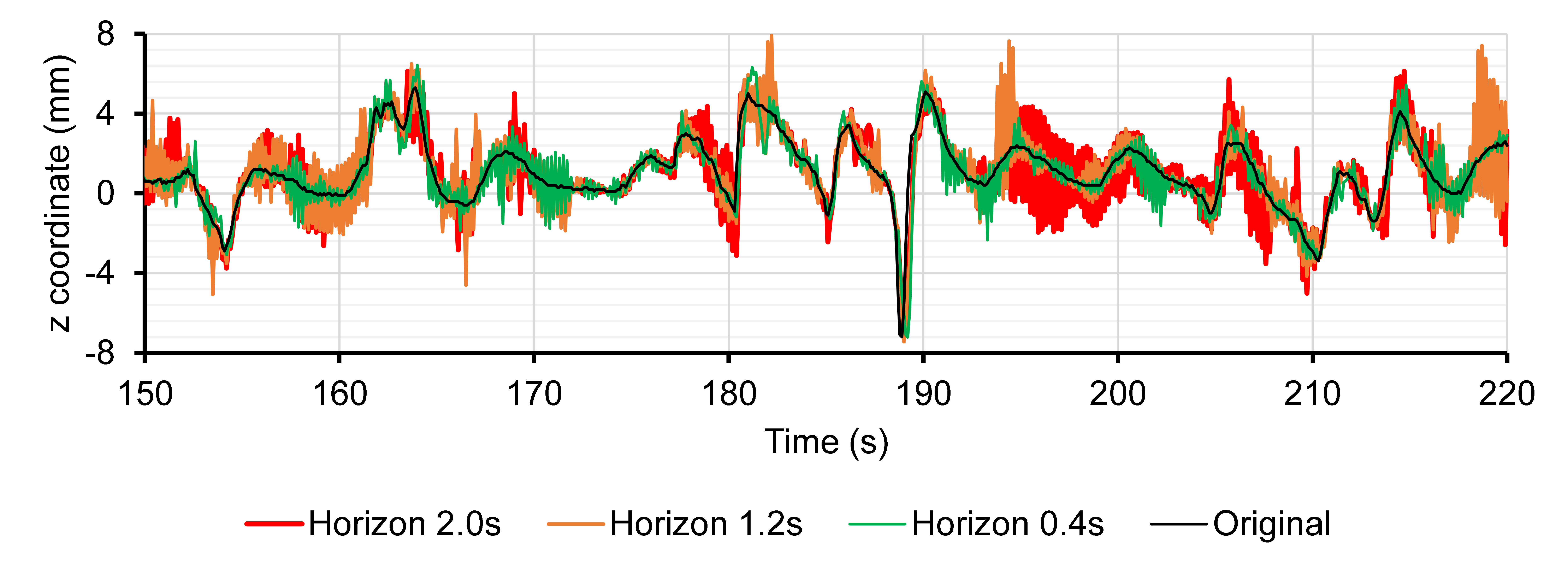
Let's first visually and qualitatively examine the predicted motion of marker 3 in sequence 1 (irregular breathing) along the spine direction for different horizon values.

The graphs below seem to indicate that UORO is more precise than RTRL and least mean squares (LMS). Indeed, we limited the number of hidden units and SHL associated with RTRL to keep an acceptable computing time. Furthermore, LMS is an adaptive linear filter that does not have the representational power of RNNs.

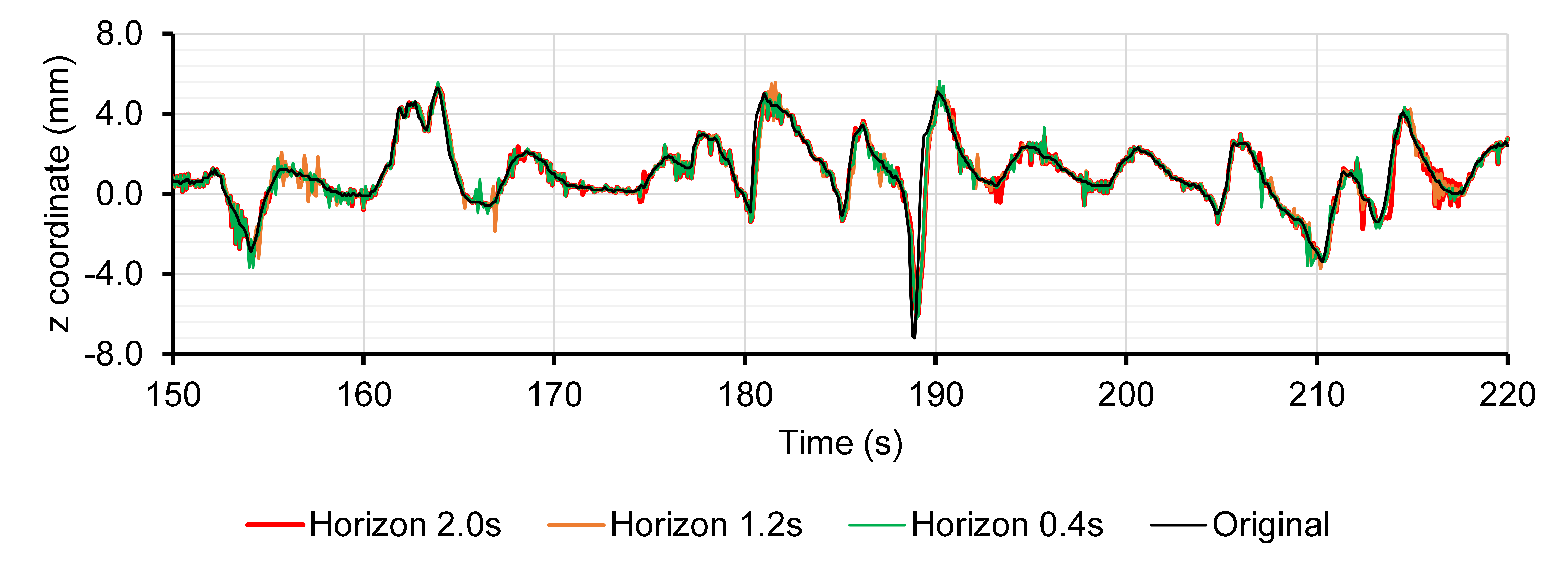
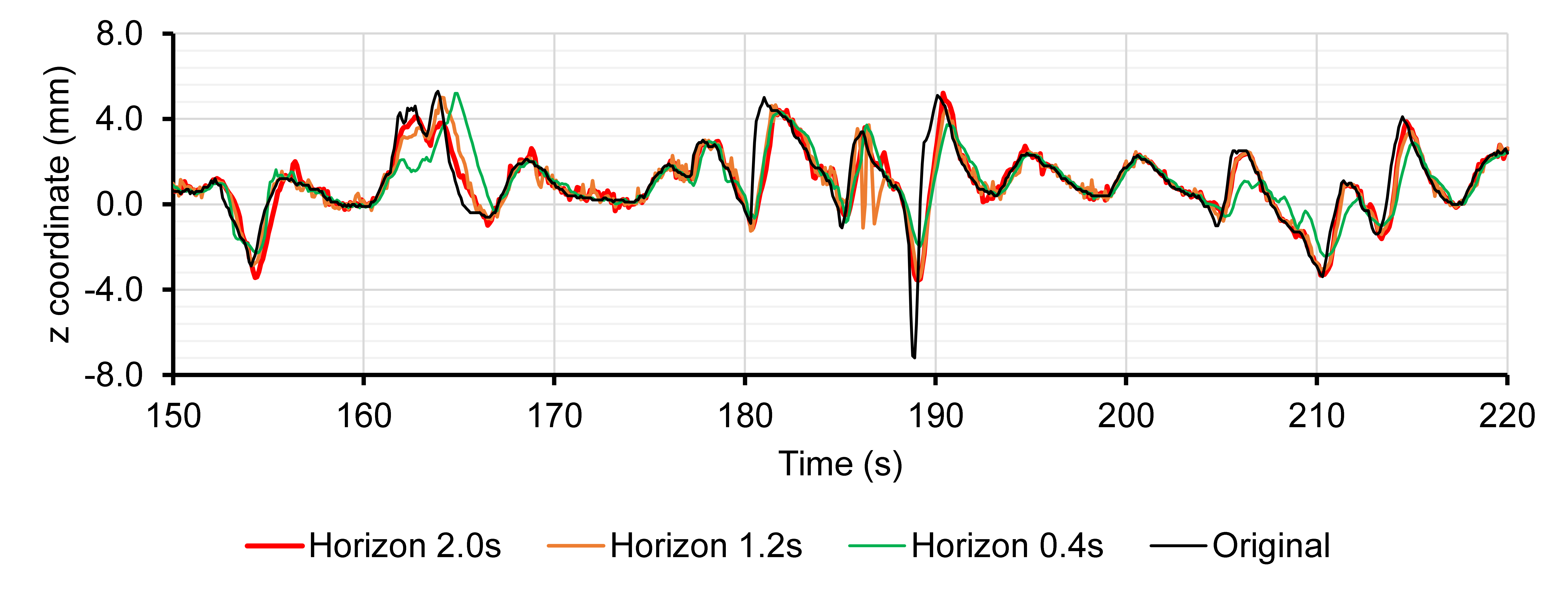
We observe that the prediction given by LMS has a high jitter, i.e., it oscillates a lot around the ground-truth marker coordinate.

3.2. Numerical forecasting accuracy

I confess that I picked the particular example above because it makes UORO look good. Still, in some situations, UORO does not perform as well as the other methods. So let's look closely at what happens when we average numerical precision metrics over horizon values between 0.1s and 2.0s and the nine sequences. Indeed, it was reported previously that the range of latencies in radiotherapy is somewhere 0.1s and 2.0s [9].

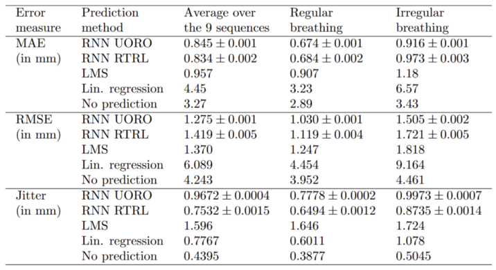
I reported several metrics as they give different information about the forecasting behavior of each algorithm. The mean average error (MAE) is the average absolute error over time stricto sensu, the root-mean-square error (RMSE) penalizes more high deviations, and the jitter measures the oscillation amplitude of the predicted signal. Predictions that oscillate much are not desirable because they make controlling the robot guiding the radiation beam more complex.

When looking at the error metrics averaged over the nine sequences, we observe that RTRL beats UORO when it comes to the MAE, but the situation is the opposite when looking at the RMSE. LMS has relatively good precision, but its jitter is high. Of course, the errors are lower when considering only the sequences corresponding to regular breathing and higher when looking at those corresponding to irregular breathing.

But different systems have different latency times. The choice of the best algorithm in each scenario depends on the latency of the radiotherapy system considered. Therefore, I plotted the forecasting errors as a function of the horizon values h.

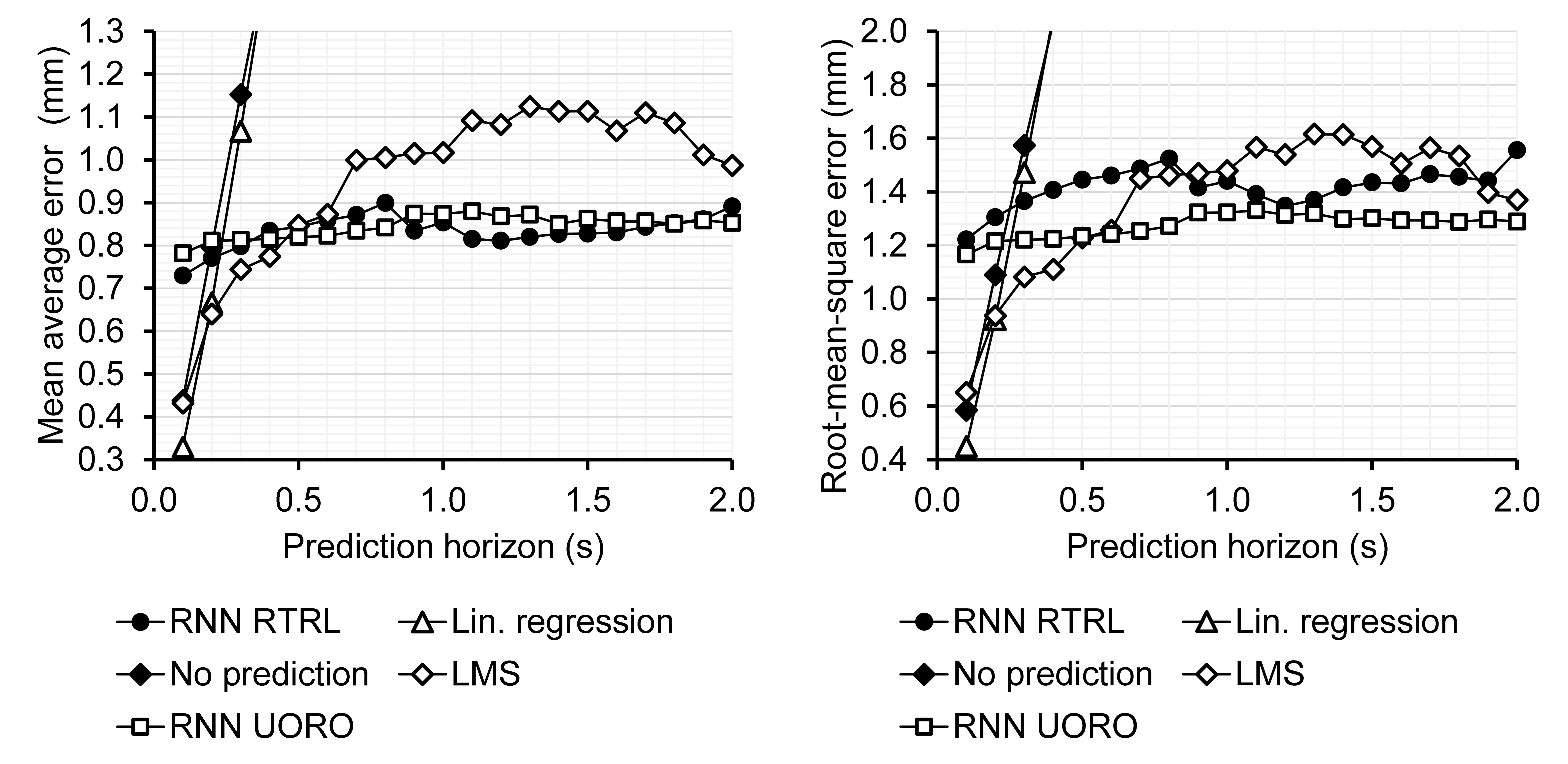
The graphs appear to have local irregularities because hyper-parameter optimization leads to different hyper-parameter choices for different values of h. However, the errors globally tend to increase as h increases. We observe that linear prediction is actually the most accurate forecasting algorithm for low values of h. LMS also appears to be efficient for intermediate values of h.

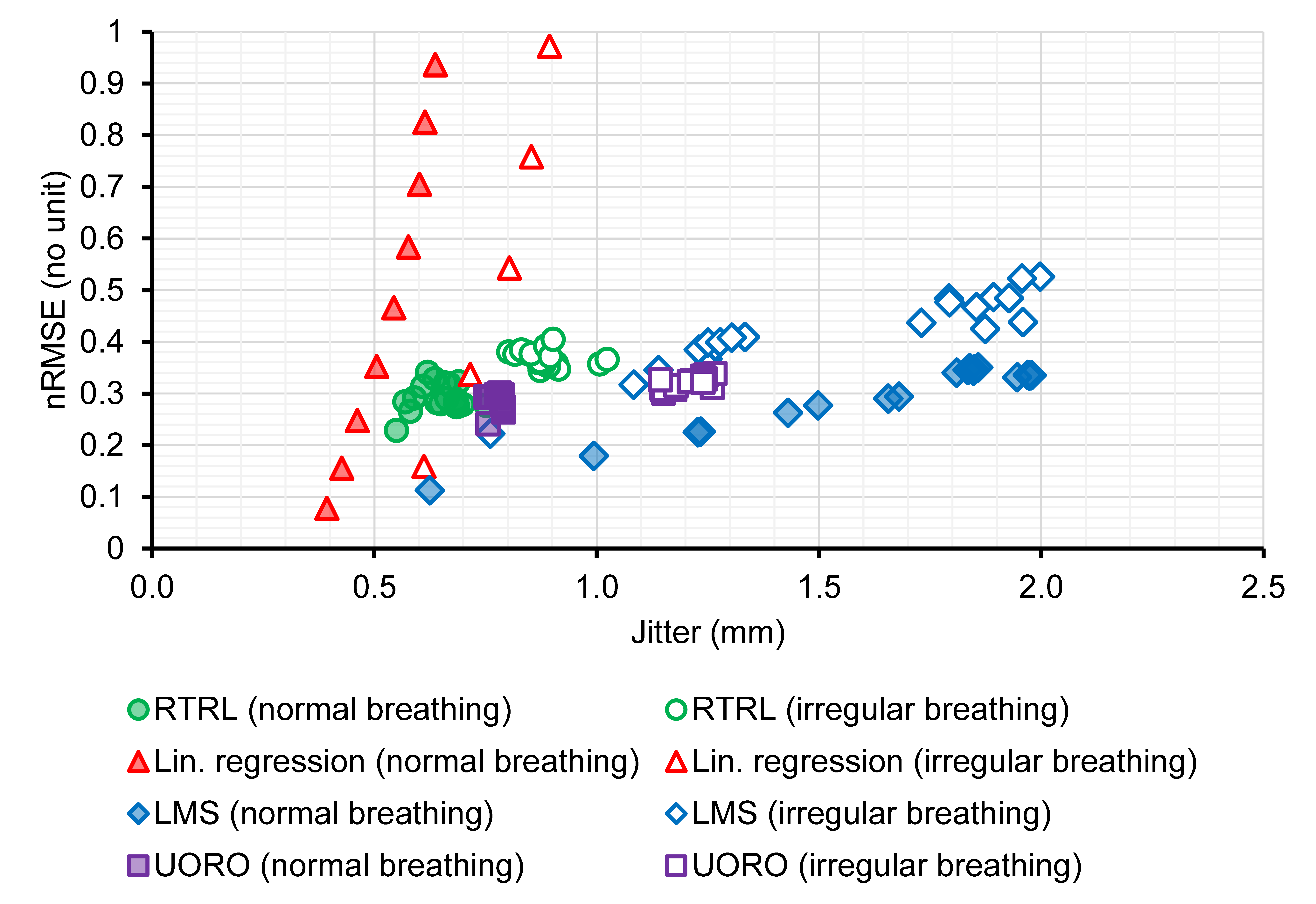
The following graph summarizes the performance of each algorithm in terms of RMSE and jitter. As a side note, in my original article, I used a similar graph describing performance in terms of "normalized RMSE," abbreviated as nRMSE, instead of RMSE; the former is a measure additionally taking into account the amplitudes of the signals when evaluating performance. Again, we observe that both the RMSE and jitter are higher for signals corresponding to irregular breathing. This 2D representation can help find the algorithm with the highest forecasting accuracy given an acceptable jitter level and a specific horizon value.

3.3. Hyper-parameter optimization

Let's talk about hyper-parameter optimization. We indicated earlier that we used cross-validation to select the network hyper-parameters leading to the best performance. I found that the learning rate and SHL were those having the strongest influence on performance in this study. So let's have a close look at how their selection impacts forecasting accuracy.

We observe again that the higher the horizon h, the higher the prediction error. In the case of high values of h, the network appears more efficient with a higher learning rate and lower SHL. In other words, in that scenario, the network works better when taking into account only the most recent signals and adapting the weights faster when changes in the incoming respiratory patterns occur.

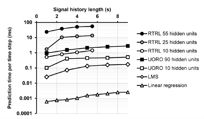
3.4. Time performance

Calculation time is one of the most important criteria for evaluating our algorithms. We observe that the prediction time increases with the SHL, which is proportional to the input layer size, and the number of hidden units. Linear regression appears to be the fastest forecasting method, followed by LMS. UORO was able to perform forecasting approximately 100 times faster than RTRL on my machine, which is a direct consequence of their respective computational complexity O(q²) and O(q⁴).

4. In short

This work is the first application of RNNs trained with UORO to respiratory motion compensation in radiotherapy. UORO is an online learning algorithm capable of learning data arriving in a streaming fashion, which enables high robustness to irregular breathing and needs fewer data than traditional learning algorithms. As a result, it has the potential to reduce irradiation of healthy tissues and, in turn, avoid side effects such as pneumothorax.

To the best of our knowledge, we used the most extensive range of horizon values h to compare the different forecasting algorithms among the studies in the literature about respiratory motion prediction. We found that linear regression achieved the lowest RMSE for 0.1s ≤ h ≤ 0.2s, followed by LMS for 0.3s ≤ h ≤ 0.5s, and UORO for h ≥ 0.6s, with respiratory signals sampled at 10Hz.

If this story was interesting to you, please do not hesitate to read the original research article, where I cover this topic more extensively and discuss mathematical details (the article is also the first to provide detailed calculations for some of the expressions related to the loss gradient in UORO for vanilla RNNs). The dataset and Matlab code are openly available, so you can use them for your own experiments if you wish. Please also kindly consider citing my research article if you do so.

5. Bonus: the rank-one trick

I would like to mention the core mathematical property that is the foundation of UORO, and which was first introduced in [10]. Here it is:

Given a decomposition of a matrix A as a sum of rank-one outer products

\[ A = \sum_{i=1}^n v_i w_i^T \]

, independent random signs νᵢ ∈ {-1, 1}, and a vector ρ of n positive real numbers, the following quantity

\[ \tilde{A} = \left( \sum_{i=1}^n \rho_i \nu_i v_i \right) \left( \sum_{i=1}^n \frac{\nu_i w_i}{\rho_i} \right)^T \]

satisfies:

\[ \mathbb{E} \tilde{A} = A \]

Furthermore, choosing

\[ \rho_i = \sqrt{\| w_i \| / \| v_i \|} \]

minimizes the variance of the approximation.

The first part of this property is relatively easy to proove, and results from the linearity of the expectation operator. The variance minimization part requires a more detailed analysis. While I will not make comments regarding the latter here, I would like to make a link with the Matlab implementation in section 2.3. You can look up at the code and see that the variable nu in my implementation corresponds to the vector ν above (line 30). The variables rho0 and rho1 (lines 40 and 41) correspond to the quantities ρᵢ in the formulas above. Notice also how the latter are expressed as the square root of the norm of two vectors in the code. The variable pred_par.eps_normalizer appearing around those fractions is here to guarantee numerical stability.

To derive the UORO algorithm, the rank-one trick is actually applied twice in conjunction with the equation describing the recursive update of the influence matrix ∂xₙ/∂θ (cf section 2.2). The proof details are in the original UORO paper [8].

References

1. Sung Hyuna, Jacques Ferlay, Rebecca L. Siegel, Mathieu Laversanne, Isabelle Soerjomataram, Ahmedin Jemal, and Freddie Bray, Global cancer statistics 2020: Globocan estimates of incidence and mortality worldwide for 36 cancers in 185 countries (2020), CA: A Cancer Journal for Clinicians
2. National Cancer Institute - Surveillance, Epidemiology and End Results Program, Cancer stat facts: Lung and bronchus cancer (2022) [accessed on June 15, 2021]
3. Pohl Michel, Mitsuru Uesaka, Hiroyuki Takahashi, Kazuyuki Demachi, and Ritu Bhusal Chhatkuli, Prediction of the Position of External Markers Using a Recurrent Neural Network Trained With Unbiased Online Recurrent Optimization for Safe Lung Cancer Radiotherapy (2022), Computer Methods and Programs in Biomedicine
4. Ritu Bhusal Chhatkuli, Development of a markerless tumor prediction system using principal component analysis and multi-channel singular spectral analysis with real-time respiratory phase recognition in radiation therapy (2016), PhD thesis, The University of Tokyo
5. Schweikard Achim, Hiroya Shiomi, and John Adler, Respiration tracking in radiosurgery (2004), Medical physics
6. Pohl Michel, Mitsuru Uesaka, Kazuyuki Demachi, and Ritu Bhusal Chhatkuli, Prediction of the motion of chest internal points using a recurrent neural network trained with real-time recurrent learning for latency compensation in lung cancer radiotherapy (2021), Computerized Medical Imaging and Graphics
7. Krilavicius Tomas, Indre Zliobaite, Henrikas Simonavicius, and Laimonas Jaruevicius, Predicting respiratory motion for real-time tumour tracking in radiotherapy (2016), ArXiv.org
8. Corentin Tallec and Yann Ollivier, Unbiased online recurrent optimization (2017), ArXiv.org
9. Verma Poonam, Huanmei Wu, Mark Langer, Indra Das, and George Sandison, Survey: real-time tumor motion prediction for image-guided radiation treatment (2010), Computing in Science & Engineering
10. Ollivier Yann, Corentin Tallec, and Guillaume Charpiat, Training recurrent networks online without backtracking (2015), ArXiv.org

• michel.pohl@centrale-marseille.fr
• Oxford, United Kingdom